Tiedosto:Equipotential by Zureks.png
Siirry navigaatioon
Siirry hakuun

Tämän esikatselun koko: 366 × 600 kuvapistettä. Muut resoluutiot: 146 × 240 kuvapistettä | 639 × 1 047 kuvapistettä.
Alkuperäinen tiedosto (639 × 1 047 kuvapistettä, 111 KiB, MIME-tyyppi: image/png)
| Tämä tiedosto on tiedostotietokanta Wikimedia Commonsista. Tiedot kuvaussivulta näkyvät alla. |  |
Tiedoston kuvaussivu Commonsissa |
Yhteenveto
| Kuvaus |
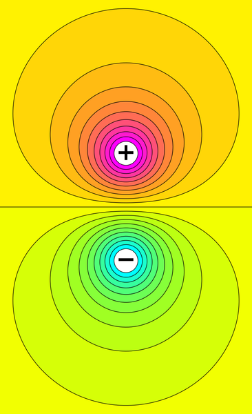
English: Voltage distribution between two electrically charged spheres (purple = positive voltage, blue = negative voltage). The black curves show equipotential contours. |
|||
| Päiväys | ||||
| Lähde | Oma teos | |||
| Tekijä | Zureks | |||
| Muut versiot |
|


Source code
The image can be created with Python Matplotlib using the following code:
import numpy as np
from matplotlib import pyplot as plt
from matplotlib import colors

cmap = colors.ListedColormap([np.clip((2*x, 2*(1-x), 4*(x-0.5)**2), 0, 1) for x in np.linspace(0., 1., 256)])

w, h = 639, 1047
xmax = 2.36
ymax = xmax * float(h) / float(w)
vmax = 0.78
y0 = 1.0
nlevels = 21
levels = np.linspace(-vmax, vmax, nlevels)
X, Y = np.mgrid[-xmax:xmax:250j, -ymax:ymax:800j]

# potential of two point charges
V  = 1.0 / np.maximum(np.sqrt(X**2 + (Y - y0)**2), 1e-2)
V -= 1.0 / np.maximum(np.sqrt(X**2 + (Y + y0)**2), 1e-2)

# rescale potential globally to make contour areas similar
V = (np.sqrt(1 + V * V) - 1) / V

plt.figure(figsize=(w/90., h/90.)).add_axes([0, 0, 1, 1])
contf = plt.contourf(X, Y, V, levels=levels, cmap=cmap,
         vmin=-vmax*(nlevels-1.)/nlevels, vmax=vmax*(nlevels-1.)/nlevels)
cont = plt.contour(X, Y, V, levels=contf.levels, colors='k', linestyles='solid')

plt.xticks([]), plt.yticks([])
plt.gca().set_aspect(aspect='equal')
plt.gca().axis('off')
plt.text(0, -y0, u'\u2212', size=48,fontweight='bold', ha='center', va='center')
plt.text(0, y0, '+', size=48,fontweight='bold', ha='center', va='center')
plt.savefig('Equipotential_of_dipole.png')
Lisenssi
| Tämä teos on saatettu Creative Commons CC0 1.0 Yleismaailmallinen Public Domain -lausuman alaisuuteen. | |
| Henkilö, joka on yhdistänyt CC0:n teokseen tai viitannut siihen teoksessa, on luovuttanut teoksen vapaaseen yleiseen käyttöön (public domain) luopumalla maailmanlaajuisesti ja soveltuvan lainsäädännön sallimassa enimmäislaajuudessa kaikista tekijänoikeuslainsäädännön alaisista oikeuksistaan teokseen, lähioikeudet ja kaikki tekijänoikeuteen liittyvät oikeudet mukaan lukien. Teosta voi lupaa pyytämättä kopioida, muokata, levittää ja esittää, mukaan lukien kaupallisessa tarkoituksessa.
|
Tiedoston historia
Päiväystä napsauttamalla näet, millainen tiedosto oli kyseisellä hetkellä.
| Päiväys | Pienoiskuva | Koko | Käyttäjä | Kommentti | |
|---|---|---|---|---|---|
| nykyinen | 17. toukokuuta 2018 kello 00.09 | | 639 × 1 047 (111 KiB) | Geek3 | Replaced with analytically computed precise contour shapes. The old version which came from an FEM simulation had significant errors towards the edges, possibly because the simulation volume was chosen too small. The potential dropped much too slowly towards the image edges. In contrast, the analytic solution is very simple, as the potential is just the linear sum of two 1/r potentials. |
| 11. huhtikuuta 2010 kello 19.37 |  | 639 × 1 047 (32 KiB) | Zureks | {{Information |Description={{en|1=Voltage distribution between two electrically charged spheres (purple = positive voltage, blue = negative voltage). The black curves show equipotential contours.}} |Source={{own}} |Author=Zureks |Date=2010 |
Tiedoston käyttö
Seuraava sivu käyttää tätä tiedostoa:
Tiedoston järjestelmänlaajuinen käyttö
Seuraavat muut wikit käyttävät tätä tiedostoa:
- Käyttö kohteessa ar.wikipedia.org
- Käyttö kohteessa be-tarask.wikipedia.org
- Käyttö kohteessa cs.wikipedia.org
- Käyttö kohteessa cv.wikipedia.org
- Käyttö kohteessa fr.wikipedia.org
- Käyttö kohteessa ht.wikipedia.org
- Käyttö kohteessa kk.wikipedia.org
- Käyttö kohteessa ko.wikipedia.org
- Käyttö kohteessa no.wikipedia.org
- Käyttö kohteessa oc.wikipedia.org
- Käyttö kohteessa ru.wikipedia.org
- Käyttö kohteessa sl.wikipedia.org
- Käyttö kohteessa uk.wikipedia.org
- Käyttö kohteessa www.wikidata.org
- Käyttö kohteessa zh.wikipedia.org